

Bioassays are methods employed to estimate the effect of a given substance in living matter, and therefore they are frequently used in the pharmaceutical industry. This is essential for the determination of potency and the assurance of activity of many proteins, vaccines, complex mixtures, and products for cell and gene therapy, as well as for their role in monitoring the stability of biological products.
Application of Bioassays
- Process Development
- Process Characterization
- Product Release
- Process Intermediates
- Stability
- Qualification of Reagents
- Product Integrity
A set of steps that will help guide the analysis of a bioassay:
1. As a part of the chosen
analysis, select the subset of data to be used in the determination of the
relative potency using the pre-specified scheme. Exclude only data known to
result from technical problems such as contaminated wells, non-monotonic
concentration–response curves, etc.
2. Fit the statistical model for
detection of potential outliers, as chosen during development, including any
weighting and transformation. This is done first without assuming similarity of
the Test and Standard curves but should include important elements of the
design structure, ideally using a model that makes fewer assumptions about the
functional form of the response than the model used to assess similarity.
3. Determine which potential
outliers are to be removed and fit the model to be used for suitability
assessment. Usually, an investigation of outlier cause takes place before
outlier removal. Some assay systems can make use of a statistical
(non-investigative) outlier removal rule, but removal on this basis should be
rare. One approach to “rare” is to choose the outlier rule so that the expected
number of false positive outlier identifications is no more than one; e.g., use
a 1% test if the sample size is about 100. If a large number of outliers are
found above that expected from the rule used, that calls into question the
assay.
4. Assess system suitability.
System suitability assesses whether the assay Standard preparation and any
controls behaved in a manner consistent with past performance of the assay. If
an assay (or a run) fails system suitability, the entire assay (or run) is
discarded and no results are reported other than that the assay (or run)
failed. Assessment of system suitability usually includes adequacy of the fit
of the model used to assess similarity. For linear models, adequacy of the
model may include assessment of the linearity of the Standard curve. If the
suitability criterion for linearity of the Standard is not met, the exclusion
of one or more extreme concentrations may result in the criterion being met.
Examples of other possible system suitability criteria include background,
positive controls, max/min, max/background, slope, IC50 (or EC50), and
variation around the fitted model.
5. Assess sample suitability for
each Test sample. This is done to confirm that the data for each Test sample
satisfy necessary assumptions. If a Test sample fails sample suitability,
results for that sample are reported as “Fails Sample Suitability.” Relative
potencies for other Test samples in the assay may still be reported. Most
prominent of sample suitability criteria is similarity, whether parallelism for
parallel models or equivalence of intercepts for slope-ratio models. For
nonlinear models, similarity assessment involves all curve parameters other
than EC50 (or IC50).
6. For those Test samples in the
assay that meet the criterion for similarity to the Standard (i.e.,
sufficiently similar concentration–response curves or similar straight-line
subsets of concentrations), calculate relative potency estimates assuming
similarity between Test and Standard, i.e., by analyzing the Test and Standard
data together using a model constrained to have exactly parallel lines or
curves, or equal intercepts.
7. A single assay is often not
sufficient to achieve a reportable value, and potency results from multiple
assays can be combined into a single potency estimate. Repeat steps 1–6
multiple times, as specified in the assay protocol or monograph, before
determining a final estimate of potency and a confidence interval.
8. Construct a variance estimate
and a measure of uncertainty of the potency estimate (e.g., confidence
interval).
Bioassays Analysis Models
1. Quantitative and Qualitative
Assay Responses
2. Parallel-Line Models for
Quantitative Responses
3. Nonlinear Models for
Quantitative Responses
4. Slope-Ratio
Concentration–Response Models
5. Dichotomous (Quantal) Assays
Relative Potency Calculation
A primary assumption underlying
methods used for the calculation of relative potency is that of similarity. Two
preparations are similar if they contain the same effective constituent or same
effective constituents in the same proportions. If this condition holds, the
Test preparation behaves as a dilution (or concentration) of the Standard
preparation. Similarity can be represented mathematically as follows.
Let FT be the
concentration–response function for the Test, and let FS be the concentration–response
function for the Standard. The underlying mathematical model for similarity is:
FT(z) = FS(ρ z)
Where, z represents the
concentration and ρ represents the relative potency of the Test sample relative
to the Standard sample.
Parallel-Line Concentration Response Models
If the general concentration–response
model (Quantitative and Qualitative Assay Responses) can be made linear in x =
log (z), the resulting equation is then:
y = α + βlog(z) + e = α + βx + e,
Where, e is the residual or error
term, and the intercept, α, and slope, β, will differ between Test and
Standard.
With the parallelism (equal
slopes) assumption, the model becomes –
yS = α + βlog(z) + e = αS + βx +
e [3.2]
yT = α + βlog(ρz) + e = [α +
βlog(ρ)] + βx + e = αT + βx + e,
Where S denotes Standard, T
denotes Test, αS = α is the y-intercept for the Standard, and αT = α + βlog (ρ)
is the y-intercept for the Test.
Nonlinear Models for Quantitative Responses
Nonlinear concentration–response
models are typically S-shaped functions. They occur when the range of
concentrations is wide enough so that responses are constrained by upper and
lower asymptotes. The most common of these models is the four-parameter
logistic function as given below.
Let y denote the observed response and z the concentration. One form of the four-parameter logistic model is -

One alternative, but equivalent, form is –

The two forms correspond as
follows:
Lower asymptote: D = a0
Upper asymptote: A = a0 + d
Steepness: B = M (related to the
slope of the curve at the EC50)
Effective concentration 50%
(EC50): C = antilog (b) (may also be termed ED50).
Parallel-Curve Concentration–Response Models

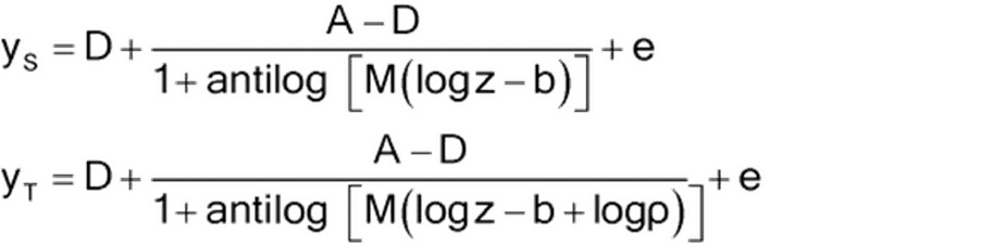
Log ρ is the log of the relative
potency and the horizontal distance between the two curves, just as for the
parallel-line model.
Slope-Ratio Concentration–Response Models
If a straight-line regression
fits the non-transformed concentration–response data well, a slope-ratio model
may be used. The equations for the slope-ratio model assuming similarity are then:
yS = α + βz + e = α + βSz + e
yT = α + β(ρz) + e = α + βSρz + e
= α + βTz + e
The model consists of one common
intercept, a slope for the Test sample results, and a slope for the Standard
sample results as in equation. The relative potency is then found from the
ratio of the slopes:
Relative Potency = Test sample
slope/Standard sample slope = βρ/β = ρ
Dichotomous (Quantal) Assays
The logit model for the probability of response, P(z), can be expressed in two equivalent forms. For the sigmoid,

Where log (ED50) = − β0/β1. An alternative form shows the relationship to linear models:
Utilizing the parameters estimated by software, which include β0, β1, and β2 and their standard errors, one obtains the estimate of the natural log of the relative potency:

Combining Independent Assays (Sample-Based Confidence Interval Methods)
Let Ri denote the logarithm of the relative potency of the ith assay of N assay results to be combined. To combine the N results, the mean, standard deviation, and standard error of the Ri are calculated in the usual way:

A variety of statistical methods
can be used to analyze bioassay data. This article presents several methods,
but many other similar methods could also be employed. Additional information
and alternative procedures can be found in the listed below and other sources:
1. Bliss CI. The Statistics of
Bioassay. New York: Academic Press; 1952.
2. Bliss CI. Analysis of the
biological assays in U.S.P. XV. Drug Stand. 1956;24:33–67.
3. Böhrer A. One-sided and two-sided
critical values for Dixon’s outlier test for sample sizes up to n = 30. Econ
Quality Control. 2008;23:5–13.
4. Brown F, Mire-Sluis A, eds.
The Design and Analysis of Potency Assays for Biotechnology Products. New York:
Karger; 2002.
5. Callahan JD, Sajjadi NC.
Testing the null hypothesis for a specified difference—the right way to test
for parallelism. Bioprocessing J. 2003:2;71–78.
6. DeLean A, Munson PJ, Rodbard
D. Simultaneous analysis of families of sigmoidal curves: application to
bioassay, radioligand assay, and physiological dose–response curves. Am J
Physiol. 1978;235:E97–E102.
7. European Directorate for the
Quality of Medicines. European Pharmacopoeia, Chapter 5.3, Statistical
Analysis. Strasburg, France: EDQM; 2004:473–507.
8. Finney DJ. Probit Analysis.
3rd ed. Cambridge: Cambridge University Press; 1971.
9. Finney DJ. Statistical Method
in Biological Assay. 3rd ed. London: Griffin; 1978.
10. Govindarajulu Z. Statistical
Techniques in Bioassay. 2nd ed. New York: Karger; 2001.
11. Hauck WW, Capen RC, Callahan
JD, et al. Assessing parallelism prior to determining relative potency. PDA J
Pharm Sci Technol. 2005;59:127–137.
12. Hewitt W. Microbiological
Assay for Pharmaceutical Analysis: A Rational Approach. New York:
Interpharm/CRC; 2004.
13. Higgins KM, Davidian M, Chew
G, Burge H. The effect of serial dilution error on calibration inference in
immunoassay. Biometrics. 1998;54:19–32.
14. Hurlbert, SH. Pseudo
replication and the design of ecological field experiments. Ecological Monogr.
1984;54:187–211.
15. Iglewicz B, Hoaglin DC. How
to Detect and Handle Outliers. Milwaukee, WI: Quality Press; 1993.
16. Nelder JA, Wedderburn RWM.
Generalized linear models. J Royal Statistical Soc, Series A. 1972;135:370–384.
17. Rorabacher DB. Statistical
treatment for rejection of deviant values: critical values of Dixon’s “Q”
parameter and related subrange ratios at the 95% confidence level. Anal Chem.
1991;63:39–48.
Related: Biological Assay Validation
Reference: USP-NF 〈1032〉, 〈1034〉
Post a Comment